More theory about Frequency Response

The frequency response is a representation of the system's open loop response to sinusoidal inputs at varying frequencies. The output of a linear system to a sinusoidal input is a sinusoid of the same frequency but with a different amplitude and phase. The frequency response is defined as the amplitude and phase differences between the input and output sinusoids. The open-loop frequency response of a system can be used to predict the behaviour of the closed-loop system .

The frequency response method may be less intuitive than other methods. However, it has certain advantages, especially in real-life situations such as modeling transfer functions from physical data. The frequency response of a system can be viewed two different ways: via the Bode plot or via the Nyquist diagram. Both methods display the same information; the difference lies in the way the information is presented.

To plot the frequency response, it is necessary to create a vector of frequencies (varying between zero (DC) and infinity) and compute the value of the system transfer function at those frequencies. If G(s) is the open loop transfer function of a system and ω is the frequency vector, we then plot G(j.ω) vs. ω. Since G(j.ω) is a complex number, we can plot both its magnitude and phase (the Bode plot) or its position in the complex plane (the Nyquist plot). Harmonic response methods can be completed using algebraic manipulation and can also be completed by testing actual systems..

Advantages

The tests involve measurements under steady state conditions which are more simpler to analyse compared to measurements of transient responses
The tests are made on open loop systems which are not subject instability problems
The results give convenient access to control system order, gain, error constants, resonant frequencies etc

Disadvantages

It is not always easy to deduce transient response characteristics from a knowledge of the frequency response
In completing tests it can be difficult to generate low-frequency signals and obtain the necessary measurements. Normal frequencies of 0,1 to 10 Hz are used. However for process control frequencies of one cycle over several hours may be required while for fluid servos frequencies of > 100 Hz may be experienced

Frequency Response Theory Using Laplace Transfer Functions

Consider a basic open loop transfer function..

The system response to a sinusoidal input is considered by providing an input signal = a. sin(ω t)

G( jω) and G(-jω) are complex values of the Open loop transfer function with s replaced by jω.

M the Magnification factor (Magnitude ratio) =y(t) / r(t). This is a function of the frequency ω.

The frequency of y(t) is the same as (r(t) but the phase is advanced by α.

A frequency response analysis (without using Laplace Transforms )

The response includes a transient response (complimentary function) and a steady state (forced) response(particular integral). In frequency response analysis only the steady state response needs to be considered. The system is linear and the output will thus be sinusoidal at a frequency ω.

If G (j ω ) = -1 ( unity gain at a phase shift of 180 ) it can be proved that the closed loop system with unity feedback will be unstable.

It can be proved that the value of ω for a value of |G(jω)| = 1 =

Phase difference between input and output =

The Nyquist plot is simply a plot of G(jω) on an argand diagram for a range of frequencies from

Frequency Response Systems Characteristics
In closed loop system , if at some frequency the signal undergoes no change in amplitude but is shifted in phase by 180 deg. ( π ) the system will be unstable. The feedback signal arriving at the summing point will reinforce the input signal and the progressive cumulative input will result in a theoretically infinite output. The feedback signal will be effectively a 100% positive feedback..

It can be therefore concluded that in the open loop version of the above system if the signal is modified resulting in unity amplitude change and a change in a phase shift of π then the system will be unstable..

In an open loop positioning control system a D.C. test signal (ω = 0) will result in the drive running continuously resulting in the output position increasing without limit. A high frequency input signal would produce zero output because the inertia of system would prevent oscillatory movement.

http://www.roymech.co.uk/Related/Control/Frequency_Response.html

Frequency Response as a Ratio of DTFTs

From Eq.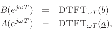 $\,$ (6.5), we have

, so that the frequency response is

$\displaystyle H(e^{j\omega T})=\frac{B(e^{j\omega T})}{A(e^{j\omega T})},$

and

$\begin{eqnarray*} B(e^{j\omega T}) &=& \mbox{{\sc DTFT}}_{\omega T}({\underline{... ...^{j\omega T}) &=& \mbox{{\sc DTFT}}_{\omega T}({\underline{a}}), \end{eqnarray*}$

where

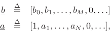
$\begin{eqnarray*} {\underline{b}}&\isdef & [b_0,b_1,\ldots,b_M,0,\ldots]\\ {\underline{a}}&\isdef & [1,a_1,\ldots,a_N,0,\ldots], \end{eqnarray*}$

and the DTFT is as defined in Eq. $\,$ (7.1).
From the above relations, we may express the frequency response of any IIR filter as a ratio of two finite DTFTs:

$\displaystyle H(e^{j\omega T}) \eqsp \frac{\mbox{{\sc DTFT}}_{\omega T}({\under... ...^M b_m e^{-j\omega mT}}{\displaystyle\sum_{n=0}^N a_n e^{-j\omega nT}} \protect$

(8.5)

This expression provides a convenient basis for the computation of an IIR frequency response in software, as we pursue further in the next section.

https://ccrma.stanford.edu/~jos/filters/Frequency_Response_Ratio_DTFTs.html

Group Delay

A more commonly encountered representation of filter phase response is called the group delay, defined by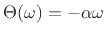

$\displaystyle \zbox {D(\omega) \isdefs - \frac{d}{d\omega} \Theta(\omega).} \qquad\hbox{(Group Delay)}$

For linear phase responses, i.e., $\Theta(\omega) = -\alpha\omega$ for some constant $\alpha$ , the group delay and the phase delay are identical, and each may be interpreted as time delay (equal to $\alpha$ samples when $\omega\in[-\pi,\pi]$ ). If the phase response is nonlinear, then the relative phases of the sinusoidal signal components are generally altered by the filter. A nonlinear phase response normally causes a ``smearing'' of attack transients such as in percussive sounds. Another term for this type of phase distortion is phase dispersion. This can be seen below in §7.6.5. An example of a linear phase response is that of the simplest lowpass filter, $\Theta(\omega) = -\omega T/2 \,\,\Rightarrow\,\, P(\omega)=D(\omega)=T/2$ . Thus, both the phase delay and the group delay of the simplest lowpass filter are equal to half a sample at every frequency.
For any reasonably smooth phase function, the group delay $D(\omega)$ may be interpreted as the time delay of the amplitude envelope of a sinusoid at frequency $\omega$ [63]. The bandwidth of the amplitude envelope in this interpretation must be restricted to a frequency interval over which the phase response is approximately linear. We derive this result in the next subsection.
Thus, the name ``group delay'' for $D(\omega)$ refers to the fact that it specifies the delay experienced by a narrow-band ``group'' of sinusoidal components which have frequencies within a narrow frequency interval about $\omega$ . The width of this interval is limited to that over which $D(\omega)$ is approximately constant.
https://ccrma.stanford.edu/~jos/filters/Group_Delay.html

Publicado por Geraldine Linares /CRF

Invite your mail contacts to join your friends list with Windows Live Spaces. It's easy! Try it!

25 Frequency Response of Integrated Circuits - conocimientos.com.ve

Páginas

domingo, 25 de julio de 2010